Introduction to Modeling and Operation of a Continuous Monoclonal Antibody (mAb) Manufacturing Process
Drugs based on monoclonal antibodies (mAbs) play an indispensable role
in biopharmaceutical industry in aspects of therapeutic and market
potentials. In therapy and diagnosis applications, mAbs are widely used
for the treatment of autoimmune diseases, and cancer, etc. According to
a recent publication, mAbs also show promising results in the treatment
of COVID-19. Until September 22, 2020,
94 therapeutic mAbs have been approved by U.S. Food & Drug
Administration (FDA) and the
number of mAbs approved within 2010-2020 is three times more than those
approved before 2010. In terms
of its market value, it is expected to reach a value of $198.2 billion
in 2023. Integrated continuous manufacturing
of mAbs represents the state-of-the-art in mAb manufacturing and has
attracted a lot of attention, because of the steady-state operations,
high volumetric productivity, and reduced equipment size and capital
cost, etc. However, there is no
existing mathematical model of the integrated manufacturing process and
there is no optimal control algorithm of the entire integrated process.
This project fills the knowledge gaps by first developing a mathematical
model of the integrated continuous manufacturing process of mAbs.
The mAb production process consists of the
upstream and the downstream processes. In the upstream process, mAb is
produced in a bioreactor which provides a conducive environment mAb
growth. The downstream process on the other hand recovers the mAb from
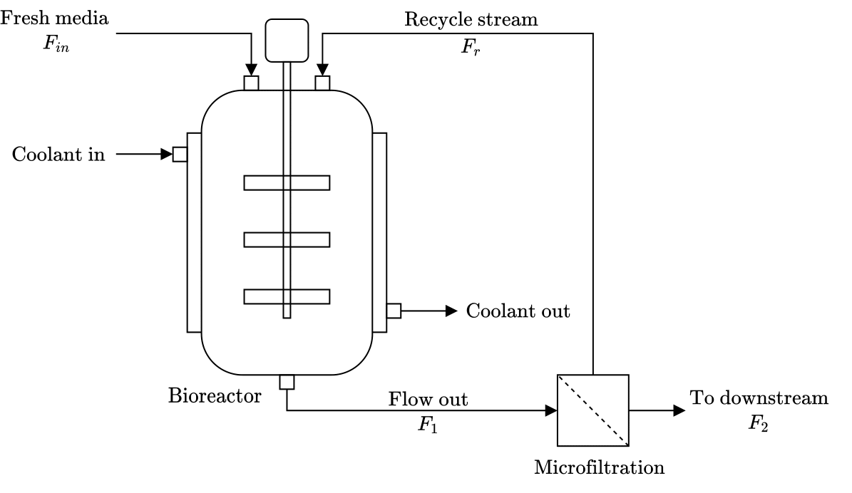
the upstream process for storage. In the upstream process for mAb
production, fresh media is fed into the bioreactor where a conducive
environment is provided for the growth of mAb. A cooling jacket in which
a coolant flows is used to control the temperature of the reaction
mixture. The contents exiting the bioreactor is passed through a
microfiltration unit which recovers part of the fresh media in the
stream. The recovered fresh media is recycled back into the bioreactor
while the stream with high amount of mAb is sent to the downstream
process for further processing. A schematic diagram of upstream process
is shown in Figure Fig. 1.
Fig. 1 A schematic diagram of the upstream process for mAb production
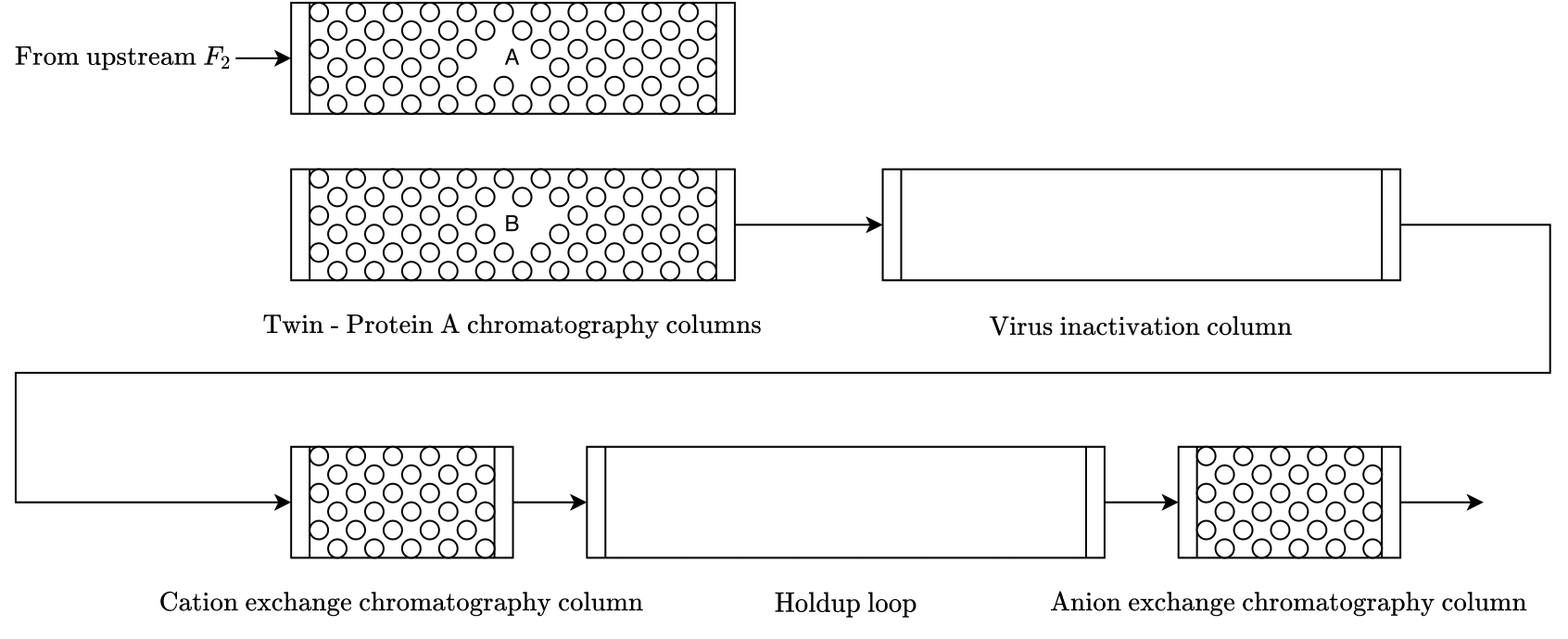
The objective of the downstream process for mAb production is to purify
the stream with high concentration of mAb from the upstream and obtain
the desired product. It is composed of a
set of fractionating columns, for separating mAb from impurities, and
holdup loops, for virus inactivation (VI) and pH conditioning. The
schematic diagram of downstream process is shown in Fig. 2.
Fig. 2 A schematic diagram of the downstream process for mAb production
There are two provided implementation of advanced
process control (APC) techniques on the operation of the upstream continuous mAb
production process,
Model Predictive Control (MAbUpstreamMPC) and Economic Model Predictive Control
(MAbUpstreamEMPC). Here we provide a brief description of both.
After conducting extensive open-loop tests, the control and prediction
horizons \(N\) for both controllers was fixed at 100. This implies
that at a sampling time of 1 hour, the controllers plan 100 hours into
the future. The weights on the deviation of the states and input from
the setpoint were identify matrices.
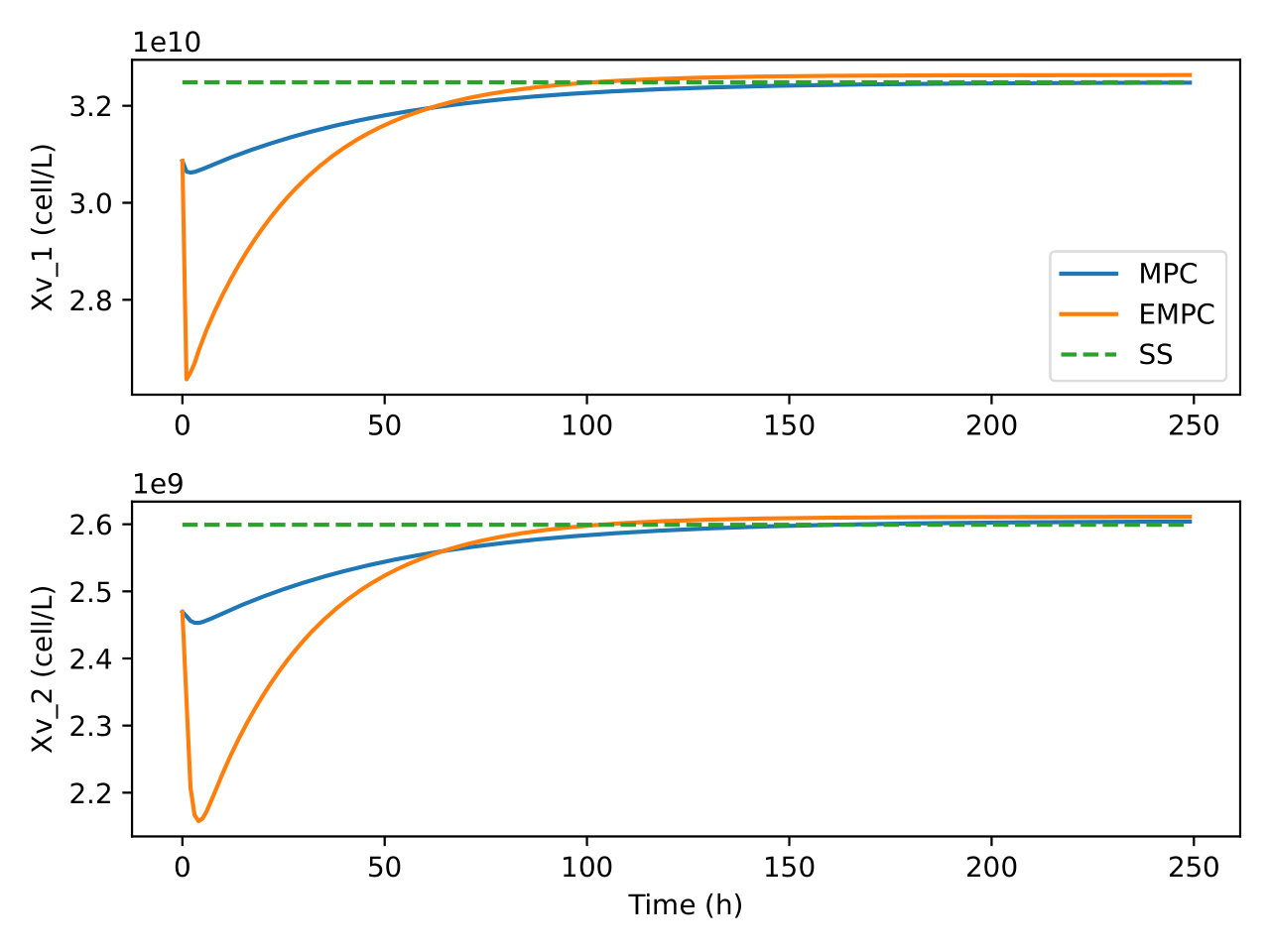
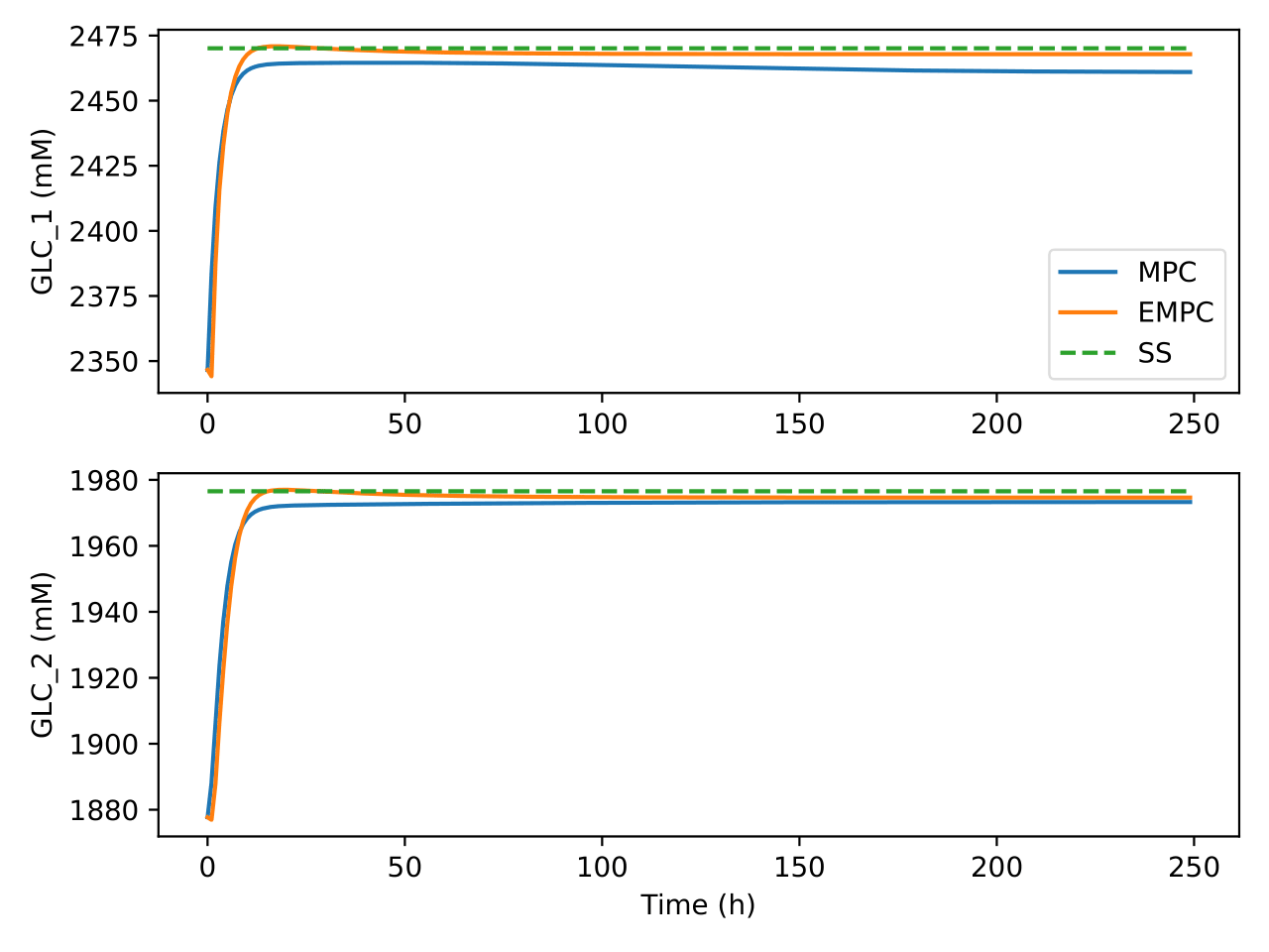
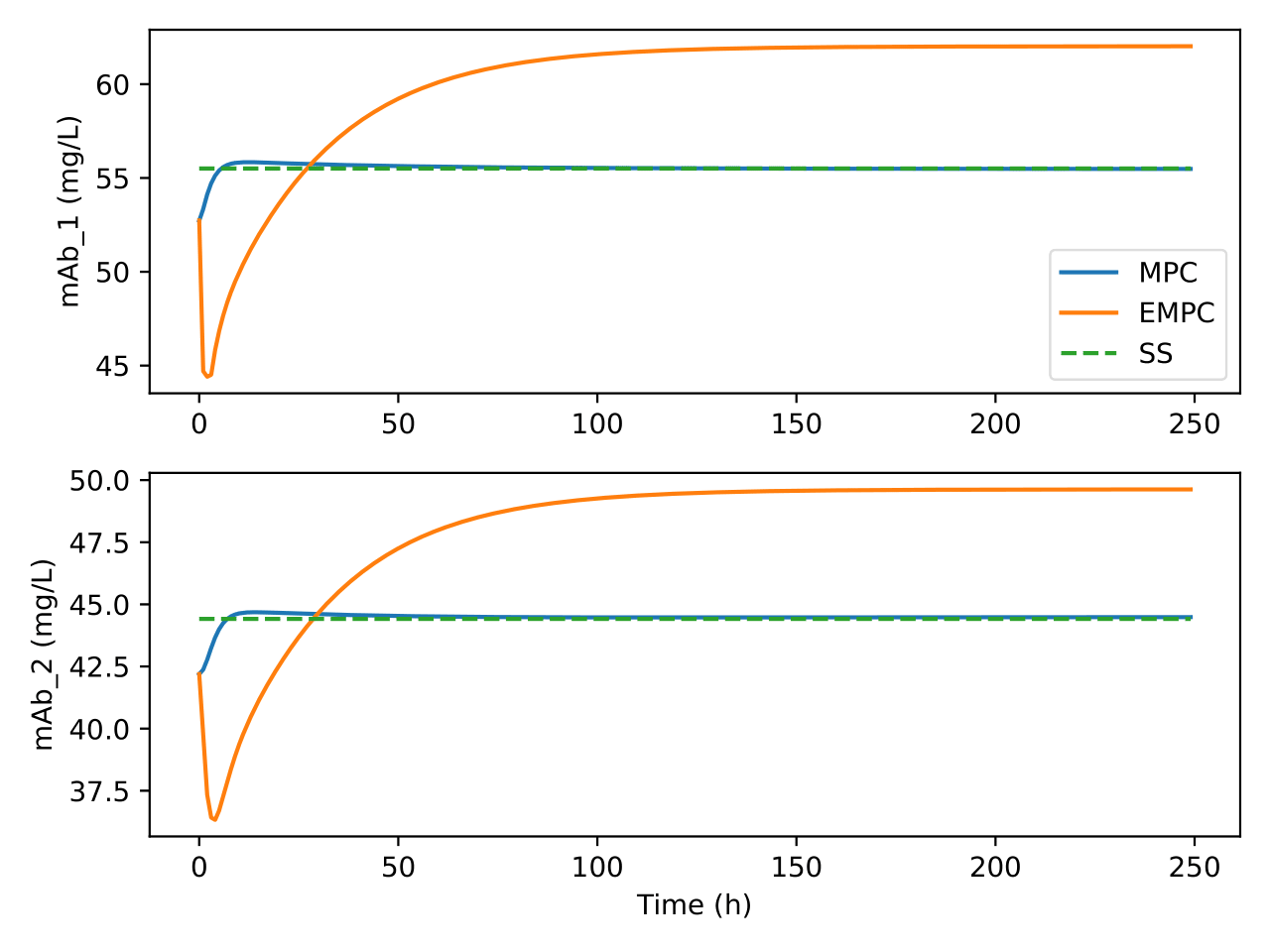
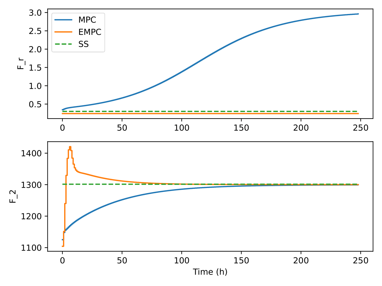
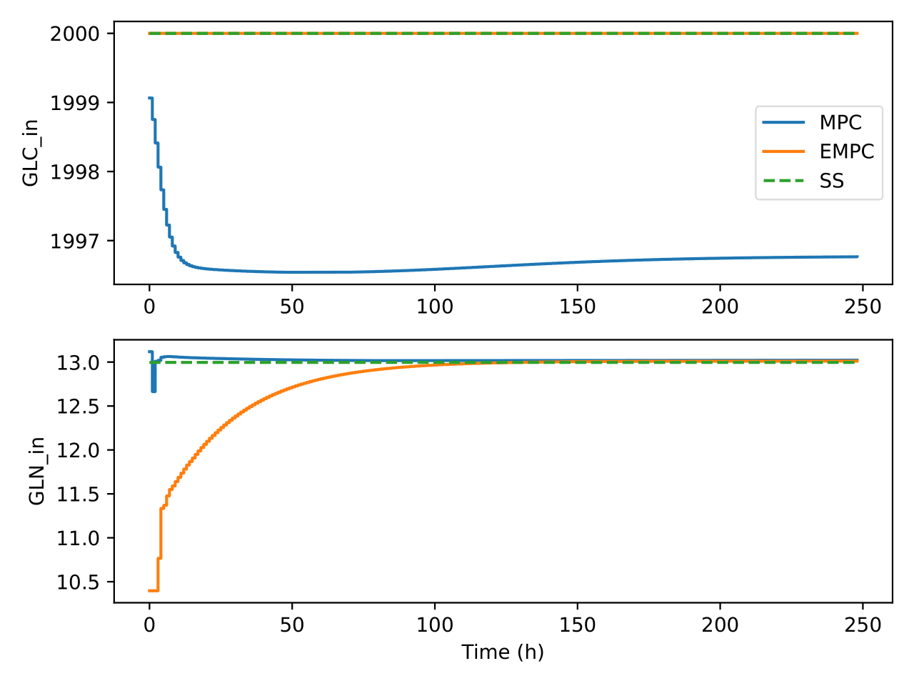
The state and input trajectories of the system under the operation of
both MPC and EMPC is shown in Figures Fig. 3 and
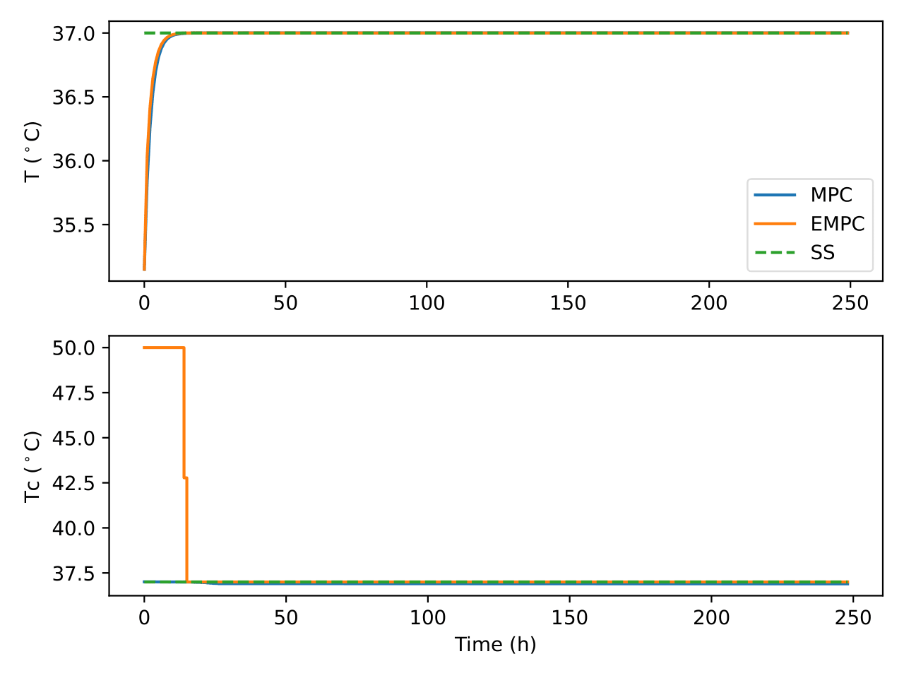
Fig. 14. It can be seen that MPC and EMPC uses
different strategies to control the process. As an example, it can be
seen in Figure Fig. 11 that EMPC initially heats up the
system before gradually reducing it whereas MPC goes to the setpoint and
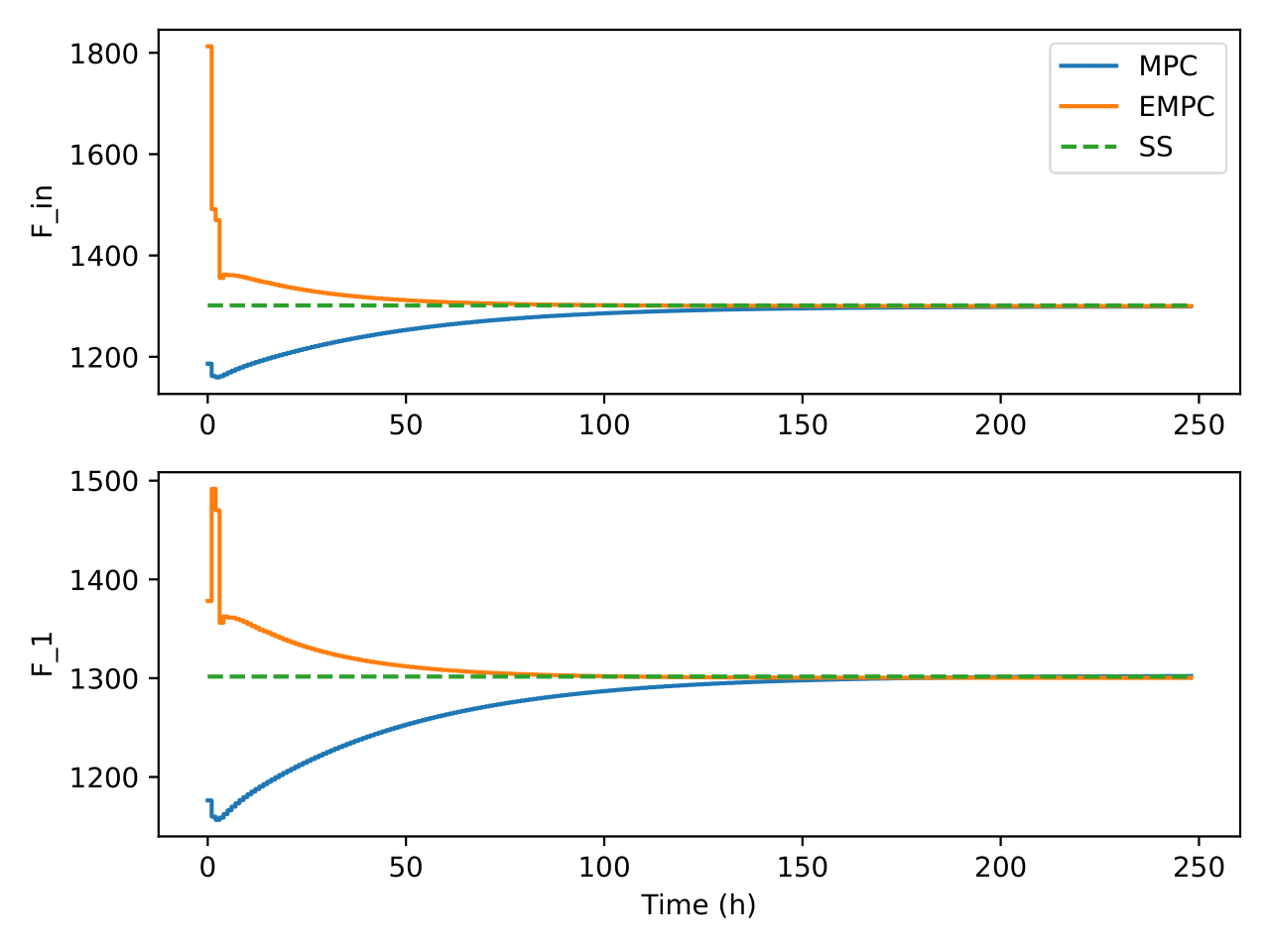
stays there. Again, EMPC tries to reduce the flow of the recycle stream
while MPC increases it as can be seen in Figure
Fig. 13. In both controllers though, the recycle
stream flow rate was kept low. Although the setpoint for the MPC was
determined under the same economic cost function used in the EMPC, it
can be seen that the EMPC does not go to that optimal steady state. This
could be due to the horizon being short for EMPC. Another possibility
could be due to numerical errors since the cost function was not scaled
in the EMPC. The cases where MPC was unable to go to the setpoint could
be due to numerical errors as a result of the large values of the states
and inputs. Further analysis may be required to confirm these
assertions.
Fig. 3 Trajectories of concentration of viable cells in the bioreactor
and separator under the two control algorithms
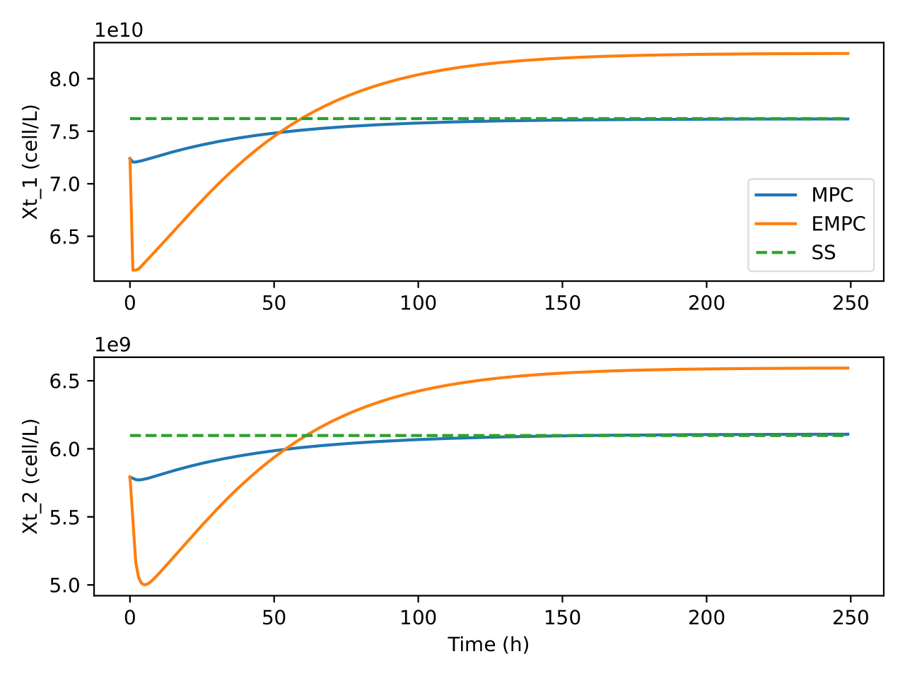
Fig. 4 Trajectories of total viable cells in the bioreactor and separator
under the two control algorithms
Fig. 5 Trajectories of glucose concentration in the bioreactor and
separator under the two control algorithms
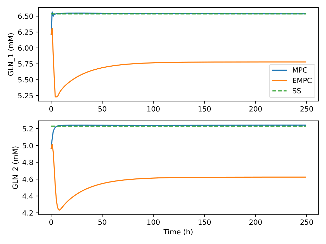
Fig. 6 Trajectories of glutamine concentration in the bioreactor and
separator under the two control algorithms
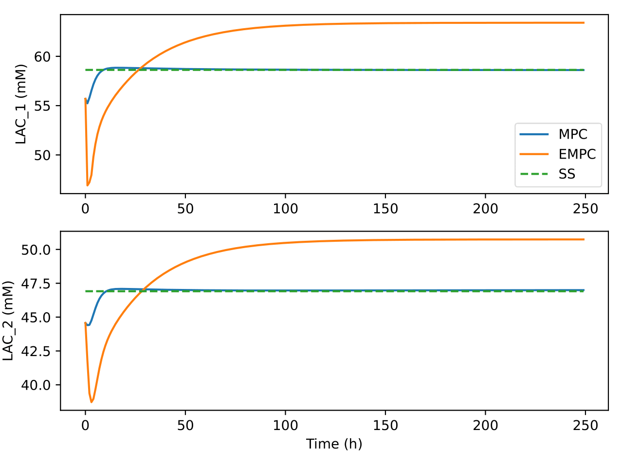
Fig. 7 Trajectories of lactate concentration in the bioreactor and
separator under the two control algorithms
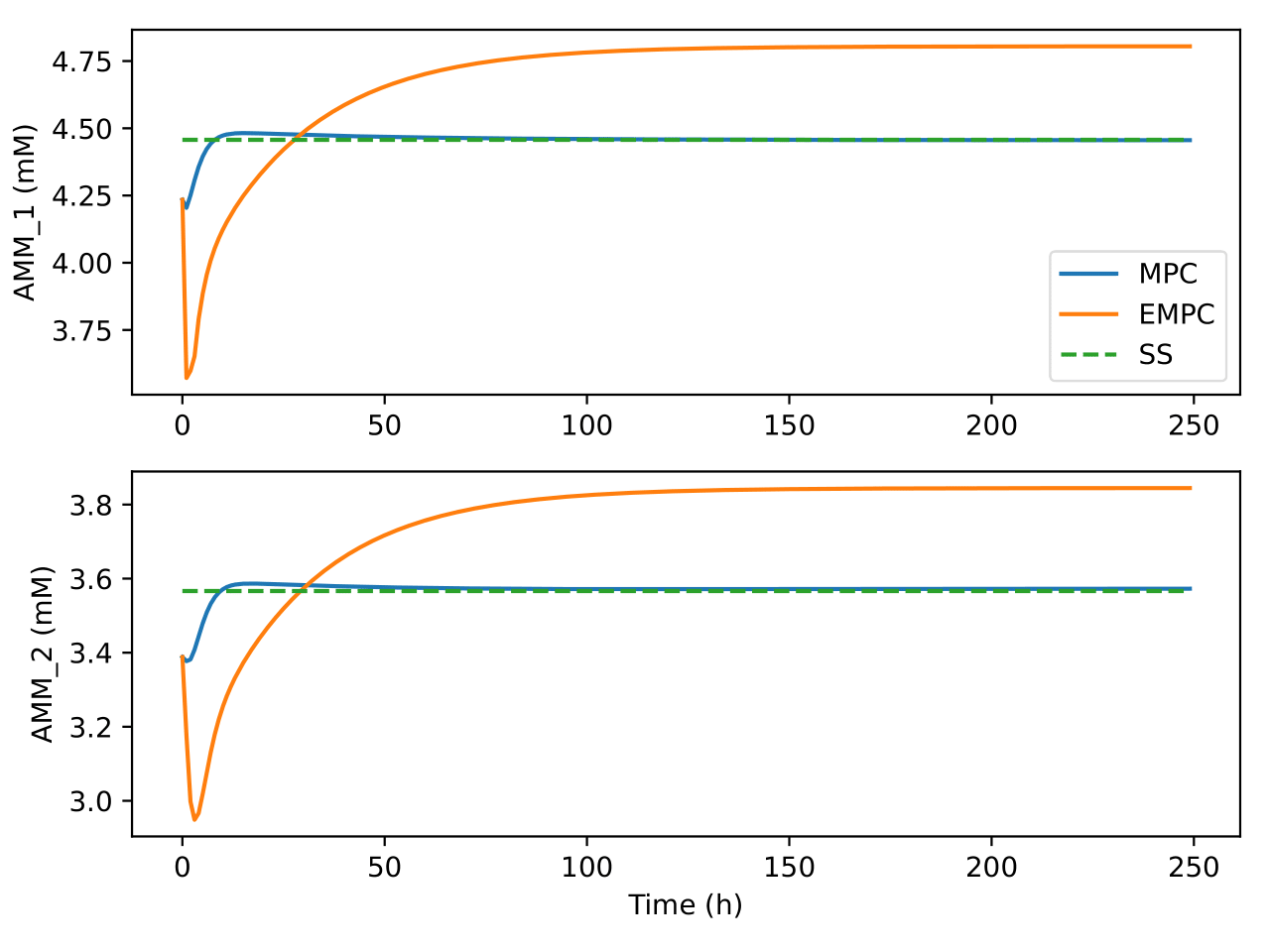
Fig. 8 Trajectories of ammonia concentration in the bioreactor and
separator under the two control algorithms
Fig. 9 Trajectories of mAb concentration in the bioreactor and separator
under the two control algorithms
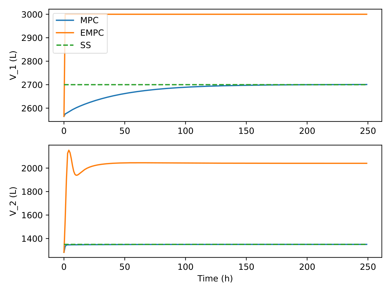
Fig. 10 Trajectories of reaction mixture volume in the bioreactor and
separator under the two control algorithms
Fig. 11 Trajectories of the bioreactor temperature and the coolant
temperature under the two control algorithms
Fig. 12 Trajectories of flow in and out of the bioreactor under the two
control algorithms
Fig. 13 Trajectories of the recycle flow rate and the flow rate out of the
upstream process under the two control algorithms
Fig. 14 Trajectories of glucose in fresh media under the two control
algorithms
The parameters of downstream model are obtained from the work of
Gomis-Fons et al and several
parameters are modified because the process is upscaled from lab scale
to industrial scale. They are summarized in
Table 6.2.
check whether the current episode is considered finished.
returns a boolean value indicated done or not, and a dictionary with information.
here in done_calculator_standard, done_info looks like {“terminal”: boolean, “timeout”: boolean},
where “timeout” is true when episode end due to reaching the maximum episode length,
“terminal” is true when “timeout” or episode end due to termination conditions such as env error encountered. (basically done)
Parameters
current_observation ([np.ndarray]) – This is denormalized observation, as usual.
returns: mean and std of rewards over all episodes.
since the rewards_list is not aligned (e.g. some trajectories are shorter than the others), so we cannot directly convert it to numpy array.
we have to convert and unwrap the nested list.
if computer_on_episodes, we first average the rewards_list over episodes, then compute the mean and std.
else, we directly compute the mean and std for each step.
when excecuting evalute_algorithms, the self.normalize should be False.
algorithms: list of (algorithm, algorithm_name, normalize). algorithm has to have a method predict(observation) -> action: np.ndarray.
num_episodes: number of episodes to run
error_reward: overwrite self.error_reward
initial_states: None, location of numpy file of initial states or a (numpy) list of initial states
to_plt: whether generates plot or not
plot_dir: None or directory to save plots
returns: list of average_rewards over each episode and num of episodes
required by gym.
This function performs one step within the environment and returns the observation, the reward, whether the episode is finished and debug information, if any.